Post-Election Model Reflection

23 November 2020 - 13 mins read time
Tags: Election 2020 Data

See the original blog post here and the forecast here.

Just days before the election, my final forecast went against the wisdom of professional forecasters and pollsters alike and projected a rail-thin electoral margin for Joe Biden. While the election results surprised many people on the night of November 3, my probabilistic model produced a point prediction with an even closer race in the electoral college–273 electoral votes for Biden compared to his actual 306–but a wider spread in the popular vote–52.8% compared to his actual 52%.

Accuracy and Patterns

The statistical aphorism that “all models are wrong, but some are useful” served as my guiding philosophy in constructing this model. As I discussed in my final prediction, I did not expect this model to perfectly forecast all outcomes in the election. Rather, this forecast aimed to provide a range of state-level probabilities and outcomes. Then, I used the most probable state-level popular vote counts to produce point predictions for the Electoral College and national popular vote. While I presented these numbers as my “final prediction”, I would have been incredibly shocked if the point predictions perfectly matched the electoral outcomes since my model’s probabilities indicated a fair amount of uncertainty.

All in all, I’m quite happy with how this model paralleled with the election outcomes. It only misclassified the winner of GA, NV, and AZ, which were three of the final states called after election night. Even though the forecast indicated that Donald Trump had a greater probability of winning these three states, the vote shares were incredibly close in the simulations, and either candidate had a fair shot of winning: Joe Biden won GA, NV, and AZ in 19.2%, 43.9%, and 20.5% of simulations, respectively.

Forecasters cannot predict the election outcome with absolute certainty, but models provide a range of possible scenarios. This model successfully anticipated a close Electoral Race with a large popular vote margin, and the actual outcome occurred more than a handful of times in my simulations.

The actual Electoral College outcome, with each candidate winning the exact combination of states that they won on Election Day, occurred in 53, or 0.001, of my simulations. To put that into perspective, the scenario from my point prediction occurred in 5080 of my simulations, which only equates to 0.051% of my simulations. With a frequentist¹ interpretation, my forecast may have correctly assigned the probabilities to each outcome and we just happened to observe one of the 53 scenarios in which each candidate won that exact grouping of states. Unfortunately, only one iteration of each election plays out in the real world, so we cannot determine the true probabilities of each outcome.

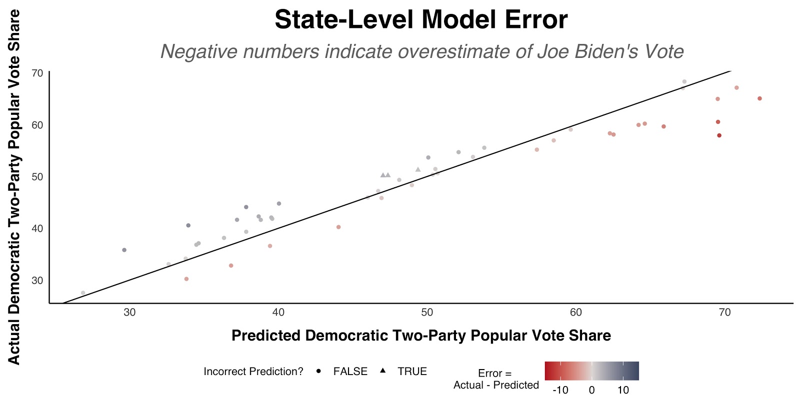
With a correlation of 0.961 between the actual and the predicted two-party popular vote for each state, the predicted state-level two-party vote shares have a very strong correlation with the actual state-level outcomes. With that said, the inaccuracies do have a couple of distinct patterns:

• On average, Joe Biden underperformed his predicted vote share by -0.242 percentage points relative to the forecast. As visible in the below scatterplot, Joe Biden’s actual vote share fell short of the model’s predictions in the Democrat-leaning states and exceeded the predicted vote share in the Republican-leaning states.

• Despite overpredicting Joe Biden’s vote share in most states, the model underestimated Joe Biden’s performance in the only three misclassified states. Essentially, the model overestimated Joe Biden’s vote share in general but underestimated it in the states with incorrect point predictions.

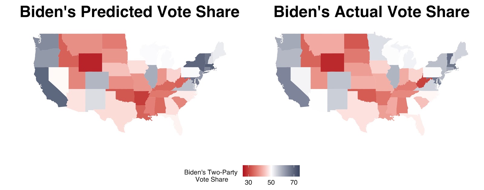
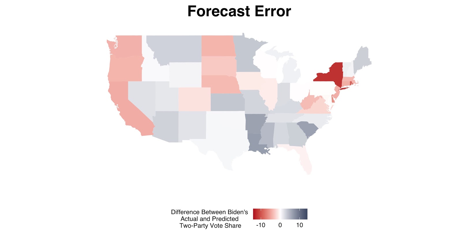
The below maps illustrate the areas with the greatest error. Notice that safe blue and red states such as New York and Louisiana have relatively large errors, while battleground states such as Texas and Ohio have extremely slim errors. The full blog post contains a table that lists all of the actual and predicted vote shares for each state.

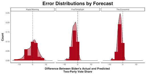
Since this model was not unilaterally biased like most other forecast models, this model’s average error is considerably closer to zero than other popular forecasts, and the errors are more normally distributed around zero:

Model	Mean Error	Root Mean Squared Error	Classification Accuracy	Missed States
Kayla Manning	-0.242	3.883	94%	AZ, GA, NV
The Economist	-2.331	2.804	96%	FL, NC
FiveThirtyEight	-2.445	3.019	96%	FL, NC

Hypotheses for Inaccuracies: Partisan Shifts in Vote Share and Voter Registration

As with any forecast model that incorporated polls, this forecast would have benefited from improved polling accuracy. Unfortunately, I do not control the polling methodology, so I must improve my model in other ways. To minimize the impact of polling biases, I applied an aggressive weighting scheme based on FiveThirtyEight’s pollster grades.² Despite these efforts, the model still produced extreme predictions in either direction, with more favorable predictions for Biden in the liberal states and more favorable predictions for Trump in conservative states. Since this model did not have a unilateral bias, I do not think polling inaccuracy is the sole culprit of my model’s shortcomings.

One hypothesis is that this model should have done a better job of detecting recent partisan shifts in vote share within the state. While the model did include lagged vote share, it did not indicate which direction a state was trending. For example, Texas voted for Trump in 2016, but the model did not know that Texas has been trending blue in recent years. The demographic variables included in my model served as a sort of proxy for such shifts, but the model did not directly include the recent partisan trends within each state. If this were the case, it would make sense why the model produced more spread out results than what played out in reality.

Does this hypothesis make sense in the context of the data we have? The model neglected to pick up on the magnitude of changing views in states such as Arizona and Georgia, both of which voted for Trump in 2016 yet voted for Biden in 2020 and were misclassified by this model.³ In addition to Georgia and Arizona, New York–the state with the largest prediction error–also followed the momentum of a 2016 partisan shift toward the center:

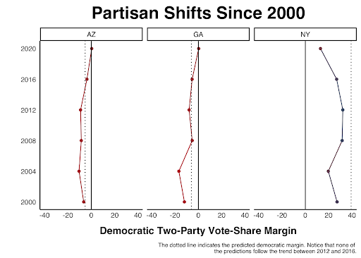
The above graphs indicate that the predictions did not align with the states’ recent partisan trends in the two-party vote share. To account for this in 2024 and beyond, I could include a variable that captures the difference in the democratic party’s two-party vote share between the two most recent elections. In this model, I attempted to use demographic changes as a proxy for this, but a more direct variable might work better.

If the trending vote shares hypothesis does not withstand quantitative assessment, I could explore other variables that measure partisan trends through other means. Changes in party registration would also pick up on changes in partisanship within a state. One benefit of party registration is that we have data for every year rather than every four years, which means the model could look at 2020 data rather than try to project from 2016. To include voter registration in the models, I could incorporate the change in Democratic voters’ percentage of the electorate from the previous election year. For example, if Democrats comprised 40% of Texas registered voters in 2016 and 45% of Texas registered voters in 2020, then the difference would be 0.45 − 0.40 = 0.05.

Proposed Test to Assess Hypotheses: Assess New Models with Additional Variables

To assess my vote share trend hypothesis, I would follow the same procedures as outlined in my final prediction to reconstruct the model with the additional variable. Once I have constructed this model, I would follow a series of steps to assess its validity:

1. First and foremost, I would assess the statistical significance of the partisan change coefficients for each of the pooled models.
2. Then, I would assess the out-of-sample fit with a leave-one-out cross-validation and compare the classification accuracy to my official 2020 forecast. If the overall accuracy is approximately equal, I would look at the yearly breakdowns and favor the model that performed better in the three most recent elections.
3. Finally, I would forecast the 2020 results using this year’s data⁴ and compare this model’s 2020 forecast to my previous model.

These assessments should provide enough metrics to determine if this new model performs better or worse than my original model in in-sample and out-of-sample validation. If this new model performed better than the original model on at least two out of these three measures, then I know that the absence of that particular variable introduced a weakness to my original model. However, if my previous model performed better or approximately the same on these measures, then I would stick with my original, more parsimonious model for the future.

To assess the validity of my voter registration hypothesis, I would follow the steps outlined above, but with the variable that captures the change in Democratic voter registration in the place of the voting shift variable. If both of these new models perform better than the original model, I would follow the same process to assess the strength of an additional model that contains both variables.

Improvements for Future Iterations

Aside from the absence of the aforementioned variables to capture partisan trends within states, I also plan to make several methodological changes to this model for the future. I touched on many of these in greater detail in my final prediction post, but here is a brief overview:

• This model does not include Washington D.C., so I manually added its 3 electoral votes after forecasting the vote shares for the 50 states. Ideally, I would find the necessary data to include D.C. in my forecast.

• Also due to the absence of appropriate data, this model allocates the electoral votes from Maine and Nebraska on a winner-take-all basis rather than following the congressional district method, as they do in reality. Again, future iterations would ideally include district-level data for these states.

• I need to improve my methodology for varying voter turnout and probabilities:
  • This model varied voter turnout and partisan probabilities independently by drawing from a normal distribution. A more sophisticated model in the future would introduce some correlation between geographies, demographic groups, and ideologies.
  • Moreover, since I drew these probabilities from a normal distribution, some states could have negative probabilities if the initial probability for voting for a particular party was extremely low (e.g. voting Republican in Hawaii). I took the absolute value of these draws to ensure all probabilities were positive, but this introduced some extreme variation in states that had an extremely low probability of voting for one party. For example, the confidence intervals for Republican votes in Hawaii were unrealistically wide since the negative vote probabilities became positive probabilities different from the positive values in the normal distributions. I must find a better method to restrict the domain in future iterations of this model.
• Lastly, I classified states based on their 2020 ideologies. In the future, I would like to set a rule for classifying each state for every election, rather than relying solely on the 2020 classification by the New York Times. For example, this model considered Colorado as a “blue state” for all years based on its 2020 classification, but it was either a “red state” or “battleground state” in most of the previous elections in the data. In its current condition, the “blue state” model was constructed with all Colorado data from 1992-2018. Ideally, I would use Colorado data from the years it was considered a “battleground state” to construct the “battleground” model, the years it was a “red state” to construct the “red” model, and the years it was a “blue state” to construct the “blue” model.

Conclusion

While my forecast failed to predict the election outcomes with absolute precision, this model correctly projected a relatively close race in the Electoral College with a larger margin in the popular vote. Furthermore, the outcomes of November 3 all reasonably match the vote shares and win probabilities estimated by the model. Even in GA, NV, and AZ–the three misclassified states–the actual vote shares were not too far from the predictions, and the simulations gave both candidates a fair probability of winning all three of those states. Despite having predicted this election exceptionally well, I hypothesize that this model’s failure to capture partisan trends within states led to the shortcomings in the predictions.

---